
文章阅读目录大纲
 https://github.com/rsharp-lang/R-sharp
降维是将数据由高维约减到低维的过程而用来揭示数据的本质低维结构。它作为克服“维数灾难”的途径在这些相关领域中扮演着重要的角色。在过去的几十年里,有大量的降维方法被不断地提出并被深入研究,其中常用的包括传统的降维算法如PCA和MDS;流形学习算法如UMAP、t-SNE、ISOMAP、LE以及LTSA等。

Integration of bulk RNAseq with single cell RNAseq of human postnatal thymus a, Uniform manifold approximation and projection (UMAP) of the single cell RNAseq dataset available from³⁰ with integration of our 11 bulk RNAseq subsets (red diamonds). DN: CD4 CD8 double negative; DP: CD4⁺ CD8⁺; P: proliferative; Q: quiescent; T(agonist): agonist selected T cells; DP (late): Positively selected DP T cells. b, Classification of single cells to each of the 11 bulk populations by logistic regression. c, Probability that single cells are classified according to any of the bulk RNAseq samples by logistic regression.
Distinct and temporary-restricted epigenetic mechanisms regulate human αβ and γδ T cell development.
Nature Immunology volume 21, pages1280–1292 (2020). https://doi.org/10.1038/s41590-020-0747-9
数据降维介绍
对于我们的数据集,一般可以通过欧几里得距离来进行差异度的计算。而我们所经常使用的很常见的聚类算法以及机器学习算法,大部分都是基于欧几里得距离来完成的。可能我们的直觉会告诉我们,理论上只要我们的数据对象的特征数越多,我们的算法对分类结果的描述应该会越准确。但是实际的结果情况可能会有些反直觉,当特征数量越多,我们的数据分类的方法在某些类型的数据集上可能失效了。这个是为什么呢?
高维空间维数灾难
现在,我们从欧几里得距离的计算公式来解释这个反直觉的结论吧。一般而言,如果我们要计算两个等长向量之间的距离的话,我们可以通过下面的欧几里得距离公式来完成:

对于高维度的数据集而言,一般是包含大量零值的稀疏矩阵。即高维空间中数据样本极其稀疏。当维数很大时,独立随机变量的和在变量规模很大时,会向其期望的和收敛,就是向一个常数收敛。这个时候根据大数定理,以欧几里得距离为基础的相对对比度将会收敛于一个常数值零:


高维空间维数灾难:高维度空间中,欧氏距离失效时任何基于欧氏距离的聚类以及机器学习算法失效
使用R#脚本进行高维空间维数灾难的验证
为了向大家展示上面所提到的欧式距离在计算高维数据时会失效这一现象,我们可以通过下面的R#脚本进行验证:
const n as integer = 500;
const raw = MNIST_LabelledVectorArray[1:n, ];
const euclidean_dimensions as function(raw) {
    str(raw);

    let d = for(i in 2:ncol(raw)) {
        const euclidean = raw[, 1:i]
        |> dist
        |> as.vector
        ;

        cat(i);
        cat("\t");

        log2((max(euclidean) - min(euclidean)) / (min(euclidean) + 0.00001));
    };

    cat("\n\n");

    d[2:length(d)] - d[1:(length(d) - 1)];
}

rownames(raw) = `X${1:n}`;

const d = euclidean_dimensions(raw);
const dims = (2:length(d))[d != 0];
const dist = data.frame(dimensions = dims, euclidean = d[d != 0]);

print(head(dist));

#         dimensions  euclidean
# <mode>  <integer>   <double>
# [1, ]   2            0.5179327
# [2, ]   3            0.1192593
# [3, ]   9            0.0760323
# [4, ]   10           0.1618553
# [5, ]   11           0.112613
# [6, ]   12           0.2113763
# [7, ]   13           0.0008718
# [8, ]   19           0.0001002
# [9, ]   20           0.060797
高维空间中大距离和小距离的差异越来越不明显
所以我们在对任何一个高维度的数据集进行分析之前,都需要进行一些适当的降维操作。
数据降维方法R#脚本示例
在这里介绍的t-SNE以及UMAP方法,都属于数据降维方法。数据降维,又可以称作为嵌入(embedding):数学上,嵌入是指一个数学结构经映射包含在另一个结构中。目前,已知的数据维度的降低方法主要有两种:
- 仅保留原始数据集中最相关的变量(特征选择)。
- 寻找一组较小的新变量,其中每个变量都是输入变量的组合,包含与输入变量基本相同的信息(降维)。
在介绍R#脚本之中的数据降维方法使用之前,我们先来了解一下方法测试所需要使用到的DEMO数据集。
简单查看测试数据集
我们在这里进行DEMO的测试数据集是来自于著名的MNIST数据集。使用的是10x10像素的已经被打好标签的图像数据,总共100个维度,6万个数据。这个数据集使用messagepack格式进行保存,我们可以使用下面的R#脚本来简单的查看一下我们的测试数据集:
imports "dataset" from "MLkit";

options("max.print" = 200);

const fileName = "MNIST-LabelledVectorArray-60000x100.msgpack";
const MNIST_LabelledVectorArray = `${dirname(@script)}/${fileName}`
|> read.mnist.labelledvector()
;

str(MNIST_LabelledVectorArray);

print(rownames(MNIST_LabelledVectorArray));

# [1]     "5" "0" "4" "1" "9" "2" "1" "3" "1" "4" "3" "5" "3"
# [14]    "6" "1" "7" "2" "8" "6" "9" "4" "0" "9" "1" "1" "2"
# [27]    "4" "3" "2" "7" "3" "8" "6" "9" "0" "5" "6" "0" "7"
# [40]    "6" "1" "8" "7" "9" "3" "9" "8" "5" "9" "3" "3" "0"
# [53]    "7" "4" "9" "8" "0" "9" "4" "1" "4" "4" "6" "0" "4"
# [66]    "5" "6" "1" "0" "0" "1" "7" "1" "6" "3" "0" "2" "1"
# [79]    "1" "7" "9" "0" "2" "6" "7" "8" "3" "9" "0" "4" "6"
# [92]    "7" "4" "6" "8" "0" "7" "8" "3" "1" "5" "7" "1" "7"
# [105]   "1" "1" "6" "3" "0" "2" "9" "3" "1" "1" "0" "4" "9"
# [118]   "2" "0" "0" "2" "0" "2" "7" "1" "8" "6" "4" "1" "6"
# [131]   "3" "4" "5" "9" "1" "3" "3" "8" "5" "4" "7" "7" "4"
# [144]   "2" "8" "5" "8" "6" "7" "3" "4" "6" "1" "9" "9" "6"
# [157]   "0" "3" "7" "2" "8" "2" "9" "4" "4" "6" "4" "9" "7"
# [170]   "0" "9" "2" "9" "5" "1" "5" "9" "1" "2" "3" "2" "3"
# [183]   "5" "9" "1" "7" "6" "2" "8" "2" "2" "5" "0" "7" "4"
# [196]   "9" "7" "8" "3" "2"
# [ reached getOption("max.print") -- omitted 59800 entries ]
测试数据集的列是数据对象的维度,行名称为数据对象的标签,总共有10种标签。我们可以通过这个数据集来测试我们的聚类算法以及分类算法的准确度。
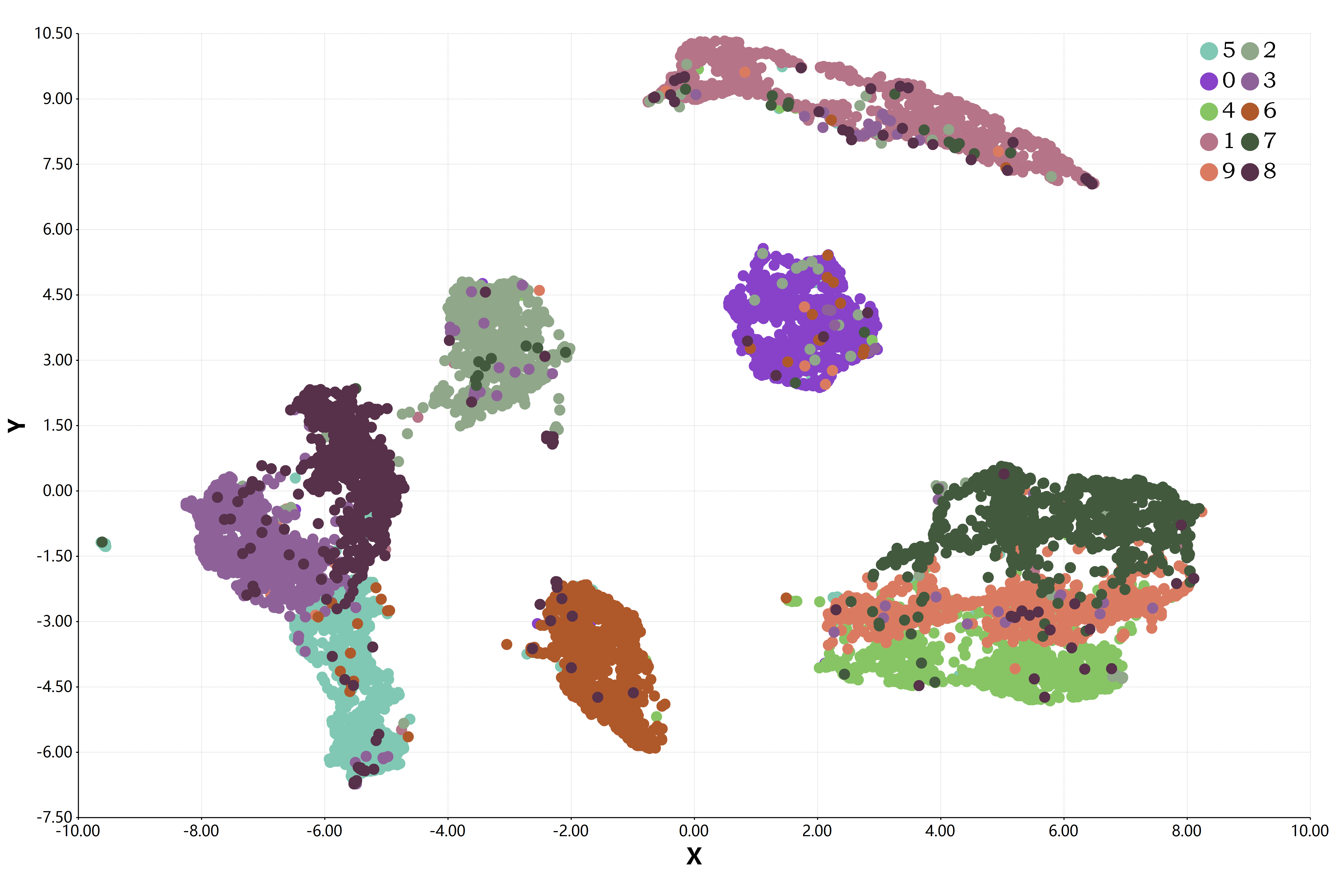
UMAP数据降维脚本
统一流形逼近与投影(UMAP,Uniform Manifold Approximation and Projection)是一种新的降维流形学习技术。UMAP是建立在黎曼几何和代数拓扑理论框架上的。UMAP是一种非常有效的可视化和可伸缩降维算法。在可视化质量方面,UMAP算法与t-SNE具有竞争优势,但是它保留了更多全局结构、具有优越的运行性能、更好的可扩展性。此外,UMAP对嵌入维数没有计算限制,这使得它可以作为机器学习的通用维数约简技术。
"Uniform Manifold Approximation and Projection (UMAP) is a dimension reduction technique that can be used for visualisation similarly to t-SNE, but also for general non-linear dimension reduction"
在下面的UMAP数据降维脚本之中,只需要一个名称为umap的核心函数来完成数据降维计算操作。
imports ["dataset", "umap"] from "MLkit";

const filename as string = "MNIST-LabelledVectorArray-60000x100.msgpack";
const MNIST_LabelledVectorArray = `${dirname(@script)}/${filename}`
|> read.mnist.labelledvector(takes = 25000)
;
const tags as string = rownames(MNIST_LabelledVectorArray);

rownames(MNIST_LabelledVectorArray) = `X${1:nrow(MNIST_LabelledVectorArray)}`;

bitmap(file = `${dirname(@script)}/MNIST-LabelledVectorArray-20000x100.umap_scatter.png`, size = [6000,4000]) {
    const manifold = umap(MNIST_LabelledVectorArray,
        dimension         = 2,
        numberOfNeighbors = 10,
        localConnectivity = 1,
        KnnIter           = 64,
        bandwidth         = 1
    )
    ;

    plot(manifold$umap,
        clusters    = lapply(tags, t -> t, names = rownames(MNIST_LabelledVectorArray)),
        labels      = rownames(MNIST_LabelledVectorArray),
        show_bubble = FALSE,
        point_size  = 50,
        legendlabel = "font-style: normal; font-size: 24; font-family: Bookman Old Style;",
        padding     = "padding:150px 150px 350px 350px;"
    );
}
一些可以调整的UMAP超参数
- n_neighbors=100, # default 15, The size of local neighborhood (in terms of number of neighboring sample points) used for manifold approximation.
- n_components=3, # default 2, The dimension of the space to embed into.
- metric='euclidean', # default 'euclidean', The metric to use to compute distances in high dimensional space.
- n_epochs=1000, # default None, The number of training epochs to be used in optimizing the low dimensional embedding. Larger values result in more accurate embeddings.
- learning_rate=1.0, # default 1.0, The initial learning rate for the embedding optimization.
- init='spectral', # default 'spectral', How to initialize the low dimensional embedding. Options are: {'spectral', 'random', A numpy array of initial embedding positions}.
- min_dist=0.1, # default 0.1, The effective minimum distance between embedded points.
- spread=1.0, # default 1.0, The effective scale of embedded points. In combination with
min_dist - low_memory=False, # default False, For some datasets the nearest neighbor computation can consume a lot of memory. If you find that UMAP is failing due to memory constraints consider setting this option to True.
- set_op_mix_ratio=1.0, # default 1.0, The value of this parameter should be between 0.0 and 1.0; a value of 1.0 will use a pure fuzzy union, while 0.0 will use a pure fuzzy intersection.
- local_connectivity=1, # default 1, The local connectivity required -- i.e. the number of nearest neighbors that should be assumed to be connected at a local level.
- repulsion_strength=1.0, # default 1.0, Weighting applied to negative samples in low dimensional embedding optimization.
- negative_sample_rate=5, # default 5, Increasing this value will result in greater repulsive force being applied, greater optimization cost, but slightly more accuracy.
- transform_queue_size=4.0, # default 4.0, Larger values will result in slower performance but more accurate nearest neighbor evaluation.
- a=None, # default None, More specific parameters controlling the embedding. If None these values are set automatically as determined by
min_distandspread - b=None, # default None, More specific parameters controlling the embedding. If None these values are set automatically as determined by
min_distandspread - random_state=42, # default: None, If int, random_state is the seed used by the random number generator;
- metric_kwds=None, # default None) Arguments to pass on to the metric, such as the
p - angular_rp_forest=False, # default False, Whether to use an angular random projection forest to initialise the approximate nearest neighbor search.
- target_n_neighbors=-1, # default -1, The number of nearest neighbors to use to construct the target simplcial set. If set to -1 use the
n_neighbors - target_metric='categorical', # default 'categorical', The metric used to measure distance for a target array is using supervised dimension reduction. By default this is 'categorical' which will measure distance in terms of whether categories match or are different.
- target_metric_kwds=None, # dict, default None, Keyword argument to pass to the target metric when performing supervised dimension reduction. If None then no arguments are passed on.
- target_weight=0.5, # default 0.5, weighting factor between data topology and target topology.
- transform_seed=42, # default 42, Random seed used for the stochastic aspects of the transform operation.
- verbose=False, # default False, Controls verbosity of logging.
- unique=False, # default False, Controls if the rows of your data should be uniqued before being embedded.
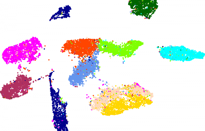
t-SNE数据降维脚本
t-Distributed Stochastic Neighbor Embedding (t-SNE)是一种降维技术,用于在二维或三维的低维空间中表示高维数据集,从而使其可视化。与其他降维算法(如PCA)相比,t-SNE创建了一个缩小的特征空间,相似的样本由附近的点建模,不相似的样本由高概率的远点建模。
在高水平上,t-SNE为高维样本构建了一个概率分布,相似的样本被选中的可能性很高,而不同的点被选中的可能性极小。然后,t-SNE为低维嵌入中的点定义了相似的分布。最后,t-SNE最小化了两个分布之间关于嵌入点位置的Kullback-Leibler(KL)散度。
t-SNE是一种集降维与可视化于一体的技术,它是基于SNE可视化的改进,解决了SNE在可视化后样本分布拥挤、边界不明显的特点,是目前较好的降维可视化手段。

在下面的一段进行t-SNE方法对100个维度的高维度数据降维的R#脚本之中,核心的函数方法只有三个函数:
- t.SNE 函数创建了一个
t-SNE - data 函数主要是用于将目标数据框对象加载进入前面的t.SNE函数所创建的计算算法对象之中
- solve 函数用于执行t-SNE降维计算,大家可以通过这个函数的iterations参数设定执行的迭代次数
在执行完t-SNE数据降维计算之后,我们就可以将结果数据导出为数据框用于后续计算分析,或者使用plot函数进行降维计算结果的可视化。
imports ["dataset", "t-SNE", "clustering"] from "MLkit";

const filename as string = "MNIST-LabelledVectorArray-60000x100.msgpack";
const MNIST_LabelledVectorArray = `${dirname(@script)}/${filename}`
|> read.mnist.labelledvector(takes = 3000)
;
const tags as string = rownames(MNIST_LabelledVectorArray);

rownames(MNIST_LabelledVectorArray) = `X${1:nrow(MNIST_LabelledVectorArray)}`;

bitmap(file = `${dirname(@script)}/MNIST-LabelledVectorArray-20000x100.t-SNE_scatter.png`, size = [6000,4000]) {
    const tSNE = t.SNE()
    |> data(MNIST_LabelledVectorArray)
    |> solve(iterations = 200)
    ;

    tSNE
    |> as.data.frame
    |> write.csv(
        file      = `${dirname(@script)}/MNIST-LabelledVectorArray-20000x100.t-SNE_scatter.csv`,
        row.names = tags
    )
    ;

    plot(tSNE,
        clusters    = lapply(tags, t -> t, names = rownames(MNIST_LabelledVectorArray)),
        labels      = rownames(MNIST_LabelledVectorArray),
        show_bubble = FALSE,
        point_size  = 50,
        legendlabel = "font-style: normal; font-size: 24; font-family: Bookman Old Style;",
        padding     = "padding:150px 150px 350px 350px;"
    );
}- 单细胞视角下的微生物基因组代谢酶嵌入分析 - 2026年2月25日
- 基因组代谢酶层级嵌入 - 2026年2月23日
- 基因组功能吉布斯LDA主题建模 - 2026年2月23日

4 Responses
[…] R#语言之中使用UMAP降维和t-SNE降维 […]
[…] 但是,使用欧几里得距离对于高维度的样本数据的计算而言,由于维度灾难的存在,对于基于欧氏距离的聚类算法在计算时间上的成本会特别高。 […]
[…] R#语言之中使用UMAP降维和t-SNE降维 […]
[…] R#语言之中使用UMAP降维和t-SNE降维 – 六月 27, 2021 […]