
文章阅读目录大纲
 https://gcmodeller.org
在这篇博客文章之中,我主要是来详细介绍一下是如何从头开始实现Phenograph单细胞分型算法的。在之前的一篇博客文章《【单细胞组学】PhenoGraph单细胞分型》之中,我们介绍了Phenograph算法的简单原理,以及一个在R语言之中所实现的Phenograph算法的程序包Rphenograph。在这里我主要是详细介绍在GCModeller软件之中所实现的VisualBasic语言版本的Phenograph单细胞分型算法。
其实,这篇博客文章也算是对之前所建立的知识点的一些总结。因为在这里Phenograph方法的实现所需要的一些知识点在之前的博客文章中都有出现过。我们首先来看一下在VisualBasic语言版本之中的Phenograph的实现代码吧:
''' <summary>
''' Jacob H. Levine and et.al. Data-Driven Phenotypic Dissection of AML Reveals Progenitor-like Cells that Correlate with Prognosis. Cell, 2015.
''' </summary>
''' <param name="data"></param>
''' <param name="k"></param>
''' <returns></returns>
Public Function CreatePhenoGraph(data As GeneralMatrix, Optional k As Integer = 30, Optional cutoff As Double = 0) As NetworkGraph
    If k < 1 Then
        Throw New ArgumentException("k must be a positive integer!")
    ElseIf k > data.RowDimension - 2 Then
        Throw New ArgumentException("k must be smaller than the total number of points!")
    End If

    message("Run Rphenograph starts:", "\n",
        "  -Input data of ", nrow(data), " rows and ", ncol(data), " columns", "\n",
        "  -k is set to ", k)

    cat("  Finding nearest neighbors...")

    ' t1 <- system.time(neighborMatrix <- find_neighbors(data, k=k+1)[,-1])
    Dim t1 As Value(Of Double) = App.ElapsedMilliseconds
    Dim neighborMatrix = ApproximateNearNeighbor _
        .FindNeighbors(data, k:=k + 1) _
        .Select(Function(row) row.indices) _
        .ToArray

    cat("DONE ~", t1 = App.ElapsedMilliseconds - CDbl(t1), "s\n", " Compute jaccard coefficient between nearest-neighbor sets...")
    ' t2 <- system.time(links <- jaccard_coeff(neighborMatrix))
    Dim t2 As Value(Of Double) = App.ElapsedMilliseconds
    Dim links As GeneralMatrix = jaccard_coeff(neighborMatrix)
    cat("DONE ~", t2 = App.ElapsedMilliseconds - CDbl(t2), "s\n", " Build undirected graph from the weighted links...")

    ' take rows
    ' colnames(relations)<- c("from","to","weight")
    ' which its coefficient should be greater than ZERO
    links = links(links(2, byRow:=False) > cutoff)

    Dim t3 As Value(Of Double) = App.ElapsedMilliseconds
    Dim g = DirectCast(links, NumericMatrix).AsGraph()
    cat("DONE ~", t3 = App.ElapsedMilliseconds - CDbl(t3), "s\n", " Run louvain clustering on the graph ...")
    Dim t4 As Value(Of Double) = App.ElapsedMilliseconds

    ' Other community detection algorithms:
    '    cluster_walktrap, cluster_spinglass,
    '    cluster_leading_eigen, cluster_edge_betweenness,
    '    cluster_fast_greedy, cluster_label_prop
    Dim community As NetworkGraph = Communities.Analysis(g)

    cat("DONE ~", t4 = App.ElapsedMilliseconds - CDbl(t4), "s\n")

    message("Run Rphenograph DONE, totally takes ", {CDbl(t1), CDbl(t2), CDbl(t3), CDbl(t4)}.Sum / 1000, "s.")
    cat("  Return a community class\n  -Modularity value:", Communities.Modularity(community), "\n")
    cat("  -Number of clusters:", Communities.Community(g).Values.Distinct.Count)

    Return community
End Function
可以看得见,光在代码层面的话,VisualBasic版本的Phenograph实现与R语言版本的Phenograph算法的实现代码是差不多的。并且在这些执行的代码中,我还对数据计算做了一些并行优化,测试下来比R语言版本的Phenograph程序包在计算效率上要提升了一大截。前面我说过了,在这篇博客文章中,是对之前所建立的知识点的一些总结。那接下来我们来看一下在这篇博客文章中我们用到了哪些之前接触过的知识点吧。
构建邻接矩阵
我们对上面所展示的代码分段的阅读下来,首先在t1阶段,最开始在Phenograph之中我们是首先要对单细胞数据集建立邻接矩阵的:
Dim neighborMatrix = ApproximateNearNeighbor _
    .FindNeighbors(data, k:=k + 1) _
    .Select(Function(row) row.indices) _
    .ToArray
在这段看似很简单的代码之中,其实底层之下,涉及到了:KNN,kd树。这段代码实现的功能就是通过KD树对每一个数据点都进行了KNN查找,基于KNN查找得到的结果,构建出了一个邻接矩阵。我们后面的图聚类就是依据这个矩阵来完成的。在R语言版本的Phenograph程序包之中,为了保证计算性能,使用的是ANN方法进行KNN的近似实现,最终实现的效果要差一些。而在GCModeller程序包中的Phenograph程序,使用的是基于KD树搜索的KNN算法实现,在单细胞的分型结果上要比ANN算法所得到的效果要好很多。
对于KD树的知识讲解,大家可以阅读之前的博客文章《【机器学习】K-D树介绍》
下面的代码展示了在底层基于kd树进行KNN查找的并行化实现:
Public Iterator Function FindNeighbors(data As IEnumerable(Of TagVector), Optional k As Integer = 30) As IEnumerable(Of (size As Integer, indices As Integer(), weights As Double()))
    Dim allData As TagVector() = data.ToArray
    Dim tree As New KdTree(Of TagVector)(allData, RowMetric(ncols:=allData(Scan0).size))
    Dim knnQuery = From row As TagVector
                   In allData.AsParallel
                   Let nn2 = tree.nearest(row, maxNodes:=k).OrderBy(Function(i) i.distance).ToArray
                   Select row.index, nn2
                   Order By index

    For Each row In knnQuery
        Dim nn2 As KdNodeHeapItem(Of TagVector)() = row.nn2
        Dim index As Integer() = nn2.Select(Function(xi) xi.node.data.index).ToArray
        Dim weights As Double() = nn2.Select(Function(xi) xi.distance).ToArray

        Yield (index.Length, index, weights)
    Next
End Function
杰卡德相关性系数计算
接下来代码执行到了t2阶段:基于KNN查找的结果,我们的单细胞数据集中的每一个数据点,都具有了一个KNN结果向量:也就是说,我们为每一个单细胞数据点都找到了组成上比较相似的其他的细胞数据点的集合。那我们接下来就可以依据这个细胞集合计算出每一个单细胞数据集之间的相似度了。对集合进行相似度的计算,我们首先想到的就是基于集合计算的杰卡德相似度。在这里我们使用的就是基于杰卡德相似度进行的相关性矩阵的建立:

''' <summary>
''' Compute jaccard coefficient between nearest-neighbor sets
'''
''' Weights of both i->j and j->i are recorded if they have intersection. In this case
''' w(i->j) should be equal to w(j->i). In some case i->j has weights while j<-i has no
''' intersections, only w(i->j) Is recorded. This Is determinded in code `if(u>0)`.
''' In this way, the undirected graph Is symmetrized by halfing the weight
''' in code `weights(r, 2) = u/(2.0*ncol - u)/2`.
''' </summary>
''' <param name="idx"></param>
''' <returns></returns>
Public Function jaccard_coeff(idx As Integer()()) As GeneralMatrix
    Dim nrow As Integer = idx.Length
    Dim weights As New List(Of Double())

    For i As Integer = 0 To nrow - 1
        For Each k As Integer In idx(i)
            If k < 0 Then
                Continue For
            End If

            Dim nodei As Integer() = idx(i)
            Dim nodej As Integer() = idx(k)
            Dim u As Integer = nodei.Intersect(nodej).Count

            If u > 0 Then
                ' symmetrize the graph
                weights.Add({i, k, u / (2.0 * nodei.Length - u) / 2})
            End If
        Next
    Next

    Return New NumericMatrix(weights.ToArray)
End Function
图聚类
在计算完杰卡德相似度矩阵之后,我们就可以得到一个两两匹配的相似度结果数据,即一个n行3列的矩阵数据。从上面所示的杰卡德相似度计算函数之中可以看得到,在这个矩阵数据之中,第一列是from节点,第二列是to节点,最后一列就是相似度作为的weight权重信息。基于这个矩阵数据,我们就可以建立起一个图对象。下面的代码演示了如何创建图对象:
Private Function AsGraph(links As NumericMatrix) As NetworkGraph
    Dim g As New NetworkGraph
    Dim from As String
    Dim [to] As String
    Dim weight As Double

    For Each row As Vector In links.RowVectors
        from = row(0)
        [to] = row(1)
        weight = row(2)

        If g.GetElementByID(from) Is Nothing Then
            Call g.CreateNode(from)
        End If
        If g.GetElementByID([to]) Is Nothing Then
            Call g.CreateNode([to])
        End If

        Call g.CreateEdge(
            u:=g.GetElementByID(from),
            v:=g.GetElementByID([to]),
            weight:=weight
        )
    Next

    Return g
End Function这个时候,程序代码执行到了t4阶段:基于louvain算法进行网络图中的节点聚类,产生网络社区集群。而这个网络社区集群就是我们的单细胞数据分型的结果。关于对louvain算法的详细讲解,大家可以阅读:《【网络可视化】基于Louvain算法的网络集群发现》。下面的代码调用实现了将目标网络图中的节点进行聚类:
Public Shared Function Analysis(g As NetworkGraph) As NetworkGraph
    Dim clusters As String() = Louvain.Builder _
        .Load(g) _
        .SolveClusters _
        .GetCommunity

    For Each v As Node In g.vertex
        v.data(NamesOf.REFLECTION_ID_MAPPING_NODETYPE) = clusters(v.ID)
    Next

    Return g
End Function
在Phenograph算法之中,对于基于图聚类产生单细胞分型的原理大家可以这样子理解:
因为相同分型的单细胞数据点,在组成成分上是相似的,所以这些数据点之前的相关性系数会非常高:因为KNN的搜索结果,这些相同分型的单细胞数据点几乎都出现在了对方的邻居列表之中,这样子基于集合运算的杰卡德相似度会很高。因为我们在完成了杰卡德相似度矩阵的建立之后,是基于这个相似度矩阵产生网络图的。所以组成上相似度很高的单细胞数据点之间相互的网络边连接会非常的丰富。这样子这些数据点在进行louvain算法聚类之后,都会更加的倾向于被划分到同一个网络集群之中。最终Phenograph算法基于此对组成上非常相似的单细胞数据点产生了一个比较符合实际情况的单细胞分型结果。
在R#
R#我将Phenograph算法模块集成在了GCModeller的phenotype_kit
imports ["geneExpression", "phenograph"] from "phenotype_kit";
require(igraph);
require(charts);
setwd(@dir);
"HR2MSI mouse urinary bladder S096_top3.csv"
|> load.expr
|> phenograph(k = 200)
|> save.network(file = "HR2MSI mouse urinary bladder S096_graph")
;
bitmap(file = `Rphenograph.png`) {
const data = read.csv("HR2MSI mouse urinary bladder S096_graph/nodes.csv", row.names = NULL);
const ID = lapply(data[, 1], function(px) as.numeric(strsplit(px, ",")));
const clusters = data[, "NodeType"];
const x = sapply(ID, px -> px[1]);
const y = sapply(ID, px -> px[2]);
plot(x, y,
class = clusters,
shape = "Square",
colorSet = "Set1:c8",
grid.fill = "white",
point_size = 25,
reverse = TRUE
);
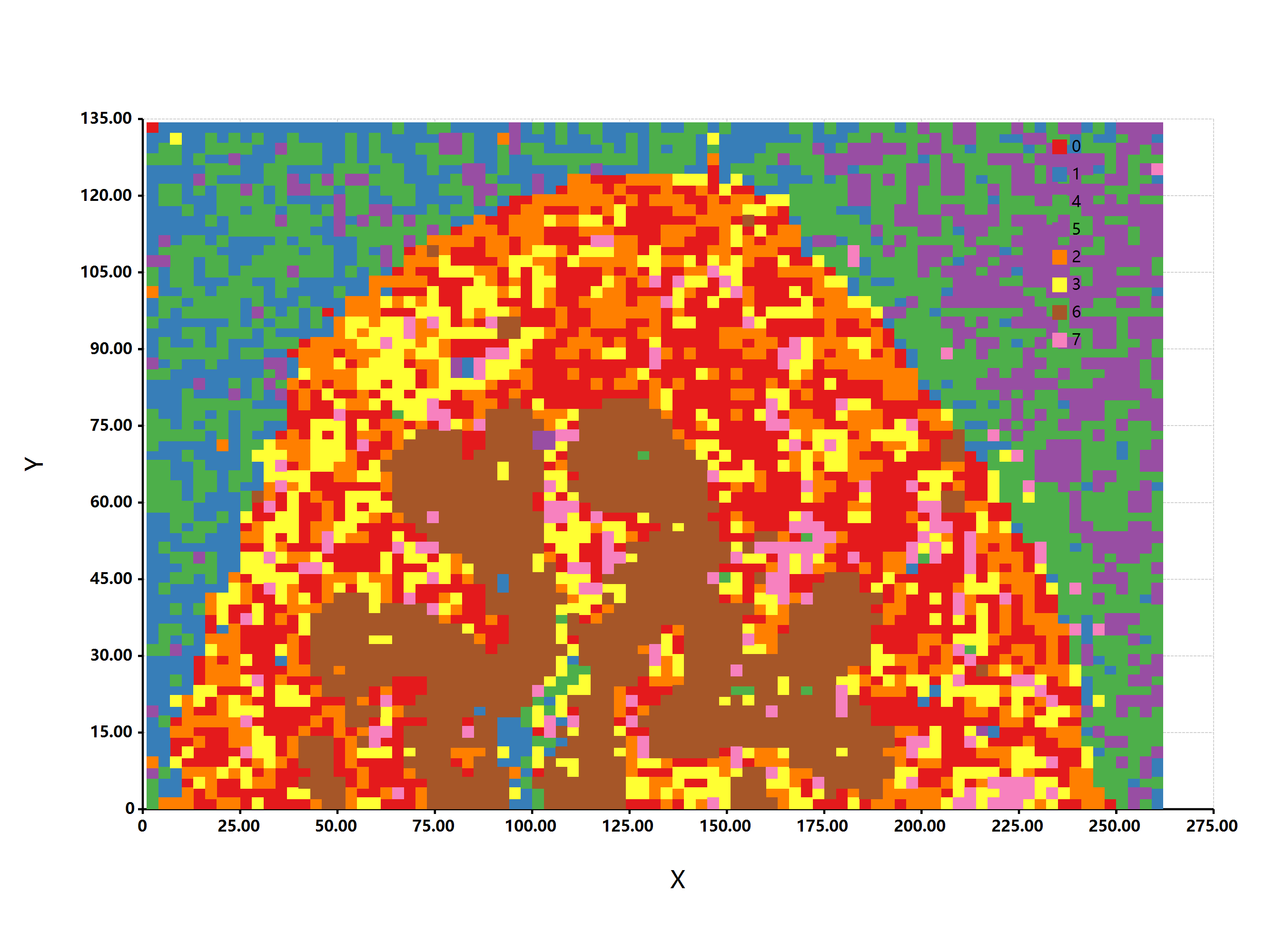
}执行一下上面的R#脚本代码,得到的分型结果还是挺符合实际的情况的:


Mass spectrometry imaging of phospholipids in mouse urinary bladder (imzML dataset)
- 单细胞视角下的微生物基因组代谢酶嵌入分析 - 2026年2月25日
- 基因组代谢酶层级嵌入 - 2026年2月23日
- 基因组功能吉布斯LDA主题建模 - 2026年2月23日

One response
There is soft rhythm in your writing, where sentences rise and fall with care. The text encourages attentive reading, reflection, and mindfulness in observing layered nuances.