
文章阅读目录大纲

LBM(格子玻尔兹曼方法)凭借其介观模型特性,在流体模拟领域展现出显著技术优势:其碰撞与迁移过程仅依赖局部数据,天然适配GPU并行计算,CUDA实现可达成10–100倍加速比;处理复杂几何边界时无需生成体网格,通过格点标记固体并配合反弹边界即可高效实现,尤其适用于多孔介质等场景;同时,通过扩展分布函数可灵活耦合多物理场,例如引入温度分布函数模拟传热,或采用伪势模型捕获多相流中的相分离现象。尽管在高速或高粘度流动中存在局限,但通过MRT算法优化及GPU硬件加速,LBM已成为微流动、多孔介质、多相流等复杂流体模拟的理想工具,在航空工程等领域已有成功应用案例,其应用前景持续拓展。
一、LBM的基本思想与理论基础
-
介观尺度特性
LBM介于微观分子动力学与宏观连续模型之间,通过统计粒子分布函数(如\(f_i(\mathbf{x},t)\))描述流体行为,而非直接求解Navier-Stokes方程。其核心是Boltzmann方程的离散化:
\[
\begin{equation}
\frac{\partial f}{\partial t} + \xi \cdot \nabla f = \Omega(f)
\end{equation}
\]
其中\(\Omega(f)\)为碰撞项,LBM通过BGK近似将其简化为:
\[
\begin{equation}
\Omega(f) \approx -\frac{1}{\tau} (f - f^{\text{eq}})
\end{equation}
\]
\(\tau\)为松弛时间,控制分布函数向平衡态\(f^{\text{eq}}\)的收敛速率。 -
离散速度模型
速度空间被离散为有限方向(如二维D2Q9模型含9个速度方向,三维D3Q19含19个方向),通过权重系数 \(w_i\) 保证宏观守恒律。以D2Q9为例:
速度方向 \(i\) \(\mathbf{c}_i\) 权重 \(w_i\) 0 (0,0) 4/9 1-4 (±1,0), (0,±1) 1/9 5-8 (±1,±1) 1/36
二、LBM核心算法流程
LBM的迭代计算分为碰撞(Collision)与迁移(Streaming)两步,辅以边界条件处理(Bounce):
- 碰撞步骤
每个格点局部更新分布函数,采用BGK模型:
\[
\begin{equation}
f_i^{\text{new}}(\mathbf{x},t) = f_i(\mathbf{x},t) - \frac{1}{\tau} \left[ f_i(\mathbf{x},t) - f_i^{\text{eq}}(\rho,\mathbf{u}) \right]
\end{equation}
\]
其中平衡态分布函数 \(f_i^{\text{eq}}\) 由宏观量(密度 \(\rho\) 、速度 \(\mathbf{u}\) )构造:
\[
\begin{equation}
f_i^{\text{eq}} = w_i \rho \left( 1 + 3\mathbf{c}_i\cdot\mathbf{u} + \frac{9}{2}(\mathbf{c}_i\cdot\mathbf{u})^2 - \frac{3}{2}\mathbf{u}^2 \right)
\end{equation}
\]
实现的vb.net代码如下所示:
Public Class collide : Inherits VectorTask

    ReadOnly cfd As FluidDynamics
    ReadOnly rho_max As Double = 1
    ReadOnly rho_min As Double = -1

    Public ReadOnly Property cpu_threads As Integer
        Get
            Return cpu_count
        End Get
    End Property

    Public Sub New(cfd As FluidDynamics)
        MyBase.New(nsize:=cfd.xdim)
        Me.cfd = cfd
    End Sub

    Protected Overrides Sub Solve(start As Integer, ends As Integer, cpu_id As Integer)
        Dim this_rho, one9thn, one36thn, vx, vy, vx2, vy2, vx3, vy3, vxvy2, v2, v215 As Double
        Dim omega = 1 / (3 * cfd.viscocity + 0.5) ' reciprocal of tau, the relaxation time

        Dim n0 As Double()
        Dim nN As Double()
        Dim nS As Double()
        Dim nE As Double()
        Dim nW As Double()
        Dim nNW As Double()
        Dim nNE As Double()
        Dim nSW As Double()
        Dim nSE As Double()

        ' Calculated variables
        Dim rho As Double()      ' macroscopic density
        Dim xvel As Double()     ' macroscopic velocity [ux]
        Dim yvel As Double()     ' macroscopic velocity [uy]
        Dim speed2 As Double()
        Dim barrier As Boolean() ' Boolean array, true at sites that contain barriers

        Const zero As Double = 0

        For x As Integer = start To ends

            n0 = cfd.n0(x)
            nN = cfd.nN(x)
            nS = cfd.nS(x)
            nE = cfd.nE(x)
            nW = cfd.nW(x)
            nNW = cfd.nNW(x)
            nNE = cfd.nNE(x)
            nSW = cfd.nSW(x)
            nSE = cfd.nSE(x)

            rho = cfd.rho(x)
            xvel = cfd.xvel(x)
            yvel = cfd.yvel(x)
            speed2 = cfd.speed2(x)
            barrier = cfd.barrier(x)

            For y As Integer = 0 To cfd.ydim - 1
                If Not barrier(y) Then
                    this_rho = n0(y) + nN(y) + nS(y) + nE(y) + nW(y) + nNW(y) + nNE(y) + nSW(y) + nSE(y)

                    If this_rho > rho_max Then
                        this_rho = rho_max
                    ElseIf this_rho < rho_min Then
                        this_rho = rho_min
                    End If

                    ' macroscopic density may be needed for plotting
                    cfd.rho(x)(y) = this_rho

                    one9thn = one9th * this_rho
                    one36thn = one36th * this_rho

                    If this_rho > zero Then
                        vx = (nE(y) + nNE(y) + nSE(y) - nW(y) - nNW(y) - nSW(y)) / this_rho
                    Else
                        vx = 0
                    End If

                    cfd.xvel(x)(y) = vx ' may be needed for plotting

                    If this_rho > zero Then
                        vy = (nN(y) + nNE(y) + nNW(y) - nS(y) - nSE(y) - nSW(y)) / this_rho
                    Else
                        vy = 0
                    End If

                    cfd.yvel(x)(y) = vy ' may be needed for plotting

                    vx3 = 3 * vx
                    vy3 = 3 * vy
                    vx2 = vx * vx
                    vy2 = vy * vy
                    vxvy2 = 2 * vx * vy
                    v2 = vx2 + vy2

                    cfd.speed2(x)(y) = v2 ' may be needed for plotting

                    v215 = 1.5 * v2
                    cfd.n0(x)(y) += omega * (four9ths * this_rho * (1 - v215) - n0(y))
                    cfd.nE(x)(y) += omega * (one9thn * (1 + vx3 + 4.5 * vx2 - v215) - nE(y))
                    cfd.nW(x)(y) += omega * (one9thn * (1 - vx3 + 4.5 * vx2 - v215) - nW(y))
                    cfd.nN(x)(y) += omega * (one9thn * (1 + vy3 + 4.5 * vy2 - v215) - nN(y))
                    cfd.nS(x)(y) += omega * (one9thn * (1 - vy3 + 4.5 * vy2 - v215) - nS(y))
                    cfd.nNE(x)(y) += omega * (one36thn * (1 + vx3 + vy3 + 4.5 * (v2 + vxvy2) - v215) - nNE(y))
                    cfd.nNW(x)(y) += omega * (one36thn * (1 - vx3 + vy3 + 4.5 * (v2 - vxvy2) - v215) - nNW(y))
                    cfd.nSE(x)(y) += omega * (one36thn * (1 + vx3 - vy3 + 4.5 * (v2 - vxvy2) - v215) - nSE(y))
                    cfd.nSW(x)(y) += omega * (one36thn * (1 - vx3 - vy3 + 4.5 * (v2 + vxvy2) - v215) - nSW(y))
                End If
            Next
        Next
    End Sub
End Class- 迁移步骤
分布函数沿离散速度方向移动到相邻格点:
\[
\begin{equation}
f_i(\mathbf{x} + \mathbf{c}_i \Delta t, t + \Delta t) = f_i^{\text{new}}(\mathbf{x},t)
\end{equation}
\]
此操作本质为数据平移,无复杂插值计算。
''' <summary>
''' *************************************************************************
'''                               - STREAM -                                 *
''' Stream particles into neighboring cells                                  *
''' From: http://physics.weber.edu/schroeder/fluids/                         *
''' **************************************************************************
''' </summary>
Friend Sub stream()
    For x As Integer = 0 To xdim - 1 - 1 ' first start in NW corner...
        For Y As Integer = ydim - 1 To 1 Step -1
            nN(x)(Y) = nN(x)(Y - 1) ' move the north-moving particles
            nNW(x)(Y) = nNW(x + 1)(Y - 1) ' and the northwest-moving particles
        Next
    Next
    For x As Integer = xdim - 1 To 1 Step -1 ' now start in NE corner...
        For Y As Integer = ydim - 1 To 1 Step -1
            nE(x)(Y) = nE(x - 1)(Y) ' move the east-moving particles
            nNE(x)(Y) = nNE(x - 1)(Y - 1) ' and the northeast-moving particles
        Next
    Next
    For x As Integer = xdim - 1 To 1 Step -1 ' now start in SE corner...
        For y As Integer = 0 To ydim - 1 - 1
            nS(x)(y) = nS(x)(y + 1) ' move the south-moving particles
            nSE(x)(y) = nSE(x - 1)(y + 1) ' and the southeast-moving particles
        Next
    Next
    For x As Integer = 0 To xdim - 1 - 1 ' now start in the SW corner...
        For y As Integer = 0 To ydim - 1 - 1
            nW(x)(y) = nW(x + 1)(y) ' move the west-moving particles
            nSW(x)(y) = nSW(x + 1)(y + 1) ' and the southwest-moving particles
        Next
    Next
    ' We missed a few at the left and right edges:
    For y As Integer = 0 To ydim - 1 - 1
        nS(0)(y) = nS(0)(y + 1)
    Next
    For y As Integer = ydim - 1 To 1 Step -1
        nN(xdim - 1)(y) = nN(xdim - 1)(y - 1)
    Next
End Sub- 边界条件处理
反弹边界:固体边界处分布函数沿入射方向反向弹回:
\[
\begin{equation}
f{\text{in}} = f{\text{out}}
\end{equation}
\]
Zou-He边界:用于速度/压力边界,通过分布函数重构强制宏观量。
热边界:温度边界通过调整分布函数值实现,如左壁加热:
\[
\begin{equation}
g_i = wi T{\text{left}} + \text{修正项}
\end{equation}
\]
Friend Sub boundary()
    ' Now handle left boundary as in Pullan's example code:
    ' Stream particles in from the non-existent space to the left, with the
    ' user-determined speed:
    Dim v = velocity
    For y As Integer = 0 To ydim - 1
        If Not barrier(0)(y) Then
            nE(0)(y) = one9th * (1 + 3 * v + 3 * v * v)
            nNE(0)(y) = one36th * (1 + 3 * v + 3 * v * v)
            nSE(0)(y) = one36th * (1 + 3 * v + 3 * v * v)
        End If
    Next
    ' Try the same thing at the right edge and see if it works:
    For y As Integer = 0 To ydim - 1
        If Not barrier(0)(y) Then
            nW(xdim - 1)(y) = one9th * (1 - 3 * v + 3 * v * v)
            nNW(xdim - 1)(y) = one36th * (1 - 3 * v + 3 * v * v)
            nSW(xdim - 1)(y) = one36th * (1 - 3 * v + 3 * v * v)
        End If
    Next
    ' Now handle top and bottom edges:
    For x As Integer = 0 To xdim - 1
        n0(x)(0) = four9ths * (1 - 1.5 * v * v)
        nE(x)(0) = one9th * (1 + 3 * v + 3 * v * v)
        nW(x)(0) = one9th * (1 - 3 * v + 3 * v * v)
        nN(x)(0) = one9th * (1 - 1.5 * v * v)
        nS(x)(0) = one9th * (1 - 1.5 * v * v)
        nNE(x)(0) = one36th * (1 + 3 * v + 3 * v * v)
        nSE(x)(0) = one36th * (1 + 3 * v + 3 * v * v)
        nNW(x)(0) = one36th * (1 - 3 * v + 3 * v * v)
        nSW(x)(0) = one36th * (1 - 3 * v + 3 * v * v)
        n0(x)(ydim - 1) = four9ths * (1 - 1.5 * v * v)
        nE(x)(ydim - 1) = one9th * (1 + 3 * v + 3 * v * v)
        nW(x)(ydim - 1) = one9th * (1 - 3 * v + 3 * v * v)
        nN(x)(ydim - 1) = one9th * (1 - 1.5 * v * v)
        nS(x)(ydim - 1) = one9th * (1 - 1.5 * v * v)
        nNE(x)(ydim - 1) = one36th * (1 + 3 * v + 3 * v * v)
        nSE(x)(ydim - 1) = one36th * (1 + 3 * v + 3 * v * v)
        nNW(x)(ydim - 1) = one36th * (1 - 3 * v + 3 * v * v)
        nSW(x)(ydim - 1) = one36th * (1 - 3 * v + 3 * v * v)
    Next
End Sub
R#
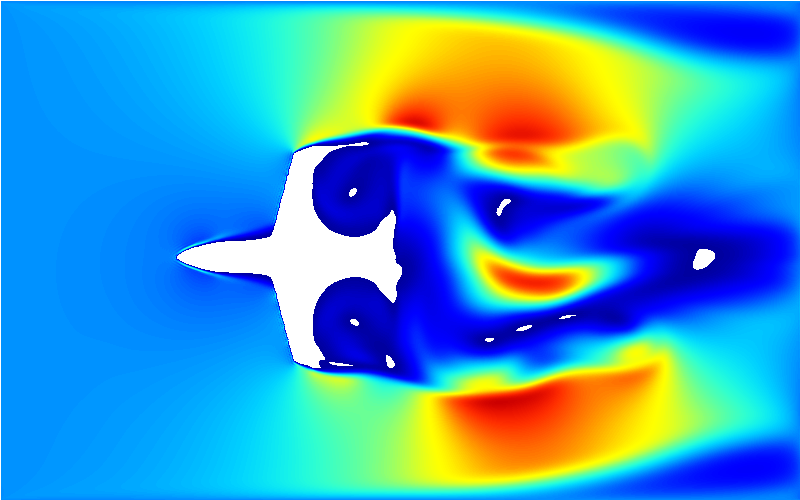
R#在下面的示例R#代码中,我们首先通过open.pack函数打开了一个用于存储CFD模拟计算结果数据的文件链接,然后再创建了一个用于CFD仿真模拟计算的运行会话。在这个会话中,我们通过加载一个png图片的方式再我们进行2D仿真计算的会话中来加载了一个喷气飞机的计算模型。
require(CFD);

let file = CFD::open.pack(relative_work("demo.dat"), mode = "write");
let dynamics = CFD::session(file, dims = [800,500],
    interval = 90,
    model.file = "../src/desktop/Daco_943767.png");

# run
CFD::start(dynamics, max.time = 20000, n_threads = 16);
close(file);
我们在这里使用一张带有透明色的喷气飞机图片来作为CFD仿真计算的模型文件。在这个文件中,所有的透明颜色都是作为空气存在,而在这张图片中,喷气飞机本身,因为没有透明像素,会在仿真模拟计算的会话中被作为障碍物处理。这样子我们就基于作为障碍物的像素分布往CFD的仿真模拟计算的环境中添加了一个具有喷气飞机外形的障碍物模型。
在下面的代码中,我们实现了流体颗粒对模型的碰撞处理:
Public Class bounce : Inherits VectorTask

    ReadOnly cfd As FluidDynamics

    Sub New(cfd As FluidDynamics)
        MyBase.New(nsize:=cfd.xdim)
        Me.cfd = cfd
    End Sub

    Protected Overrides Sub Solve(start As Integer, ends As Integer, cpu_id As Integer)
        For x As Integer = start To ends - 1
            For Y As Integer = 1 To cfd.ydim - 2
                If cfd.barrier(x)(Y) Then
                    If cfd.nN(x)(Y) > 0 Then
                        cfd.nS(x)(Y - 1) += cfd.nN(x)(Y)
                        cfd.nN(x)(Y) = 0
                    End If
                    If cfd.nS(x)(Y) > 0 Then
                        cfd.nN(x)(Y + 1) += cfd.nS(x)(Y)
                        cfd.nS(x)(Y) = 0
                    End If
                    If cfd.nE(x)(Y) > 0 Then
                        cfd.nW(x - 1)(Y) += cfd.nE(x)(Y)
                        cfd.nE(x)(Y) = 0
                    End If
                    If cfd.nW(x)(Y) > 0 Then
                        cfd.nE(x + 1)(Y) += cfd.nW(x)(Y)
                        cfd.nW(x)(Y) = 0
                    End If
                    If cfd.nNW(x)(Y) > 0 Then
                        cfd.nSE(x + 1)(Y - 1) += cfd.nNW(x)(Y)
                        cfd.nNW(x)(Y) = 0
                    End If
                    If cfd.nNE(x)(Y) > 0 Then
                        cfd.nSW(x - 1)(Y - 1) += cfd.nNE(x)(Y)
                        cfd.nNE(x)(Y) = 0
                    End If
                    If cfd.nSW(x)(Y) > 0 Then
                        cfd.nNE(x + 1)(Y + 1) += cfd.nSW(x)(Y)
                        cfd.nSW(x)(Y) = 0
                    End If
                    If cfd.nSE(x)(Y) > 0 Then
                        cfd.nNW(x - 1)(Y + 1) += cfd.nSE(x)(Y)
                        cfd.nSE(x)(Y) = 0
                    End If
                End If
            Next
        Next
    End Sub
End Class在完成了仿真计算后,针对得到的计算结果文件,接下来我们就可以通过dump_stream函数将计算得到的每一帧的数据以热图的形式导出来,在指定的文件夹中生成每一帧的数据热图结果。在进行热图渲染的时候,可以参考之前写的讲解颜色调色板的文章中列举出来的颜色版进行热图的颜色设置。
require(CFD);

relative_work("demo.dat")
|> CFD::open.pack(mode = "read")
|> CFD::dump_stream(
    fs = "/tmp/video",
    colors = "jet",
    color.levels = 200
);
最后,我们通过ffmpeg工具,将这些导出来的模拟计算的结果帧合并为视频。

ffmpeg -f image2 -r 25 -i "/tmp/video/frame-%5d.bmp" -vcodec libx264 -crf 22 ./output.mp4- 单细胞视角下的微生物基因组代谢酶嵌入分析 - 2026年2月25日
- 基因组代谢酶层级嵌入 - 2026年2月23日
- 基因组功能吉布斯LDA主题建模 - 2026年2月23日

2 Responses
Một demo mô phỏng chất lưu thật tuyệt vời! Very awesome Very awesome
thx